Sentinel-2 super-resolution and land-cover mapping
I retrained a small image-sharpening model on real satellite photo pairs. It went from worse than a standard enlargement to slightly better, on 83% of 13,039 test patches.
Published 31 Oct 2026 · Updated 1 Nov 2026
- My part
- Research review, comparison with ESA's model, the mapping experiment, retraining on real data, repo restructure and automated tests
- Team
- 3 · Shantanu Vasagadekar, Aniruddha Kadam, Shrihari Kshirsagar
- Timeline
- Oct 2026
- Status
- Finished; one experiment still to re-run with the new model
- Skills
- Python · PyTorch · RCAN · U-Net · SegFormer · rasterio / GeoTIFF · ONNX Runtime · PyQt5 · GitHub Actions
- Links
- Code · Experiment write-up
- Skills
- Computer vision, Python
In short
- Problem
- Free Sentinel-2 satellite images show 10 m per pixel, too coarse for small roads and buildings. Sharpening models often invent detail that isn't really there.
- What I did
- Found that our first model, trained on artificial examples, was worse than a plain enlargement on real images. Retrained it on real pairs of satellite photos.
- Result
- Now slightly better than a plain enlargement on 83% of 13,039 test patches. Sharper input did not make land-cover maps more accurate.
- How to check
- Code and 107 automated tests · raw results behind every number in the repo · trained model included, so the app runs on a laptop
The problem: free satellite images are 10 m, and fake detail is easy
Oct 2026
Sentinel-2 gives free images of the whole planet every few days, but at 10 m per pixel. Small roads, narrow fields and single buildings blur together. Super-resolution models promise to turn that into 5 m.
The catch is training data. There are almost no matching pairs of the same place at 10 m and 5 m on the same day. So most models are trained on artificial pairs: a sharp image blurred down by a formula. Our first model was trained that way. It produced crisp-looking output, but crisp is not the same as correct.
So the project asked two questions: does the model beat plain bicubic enlargement on real imagery, and does a sharper image make a better land-cover map?
My role: testing the model on real data, then fixing it
The project’s first version (the desktop app, a model trained on artificial data and a land-cover detector) was already in place on 12 Oct. From 22 Oct I wrote 14 of the repository’s 15 commits:
- Research review of prior work, competing tools and recent papers on satellite super-resolution.
- A fair comparison against ESA’s SEN2SR model and bicubic on 42 real Indian scenes.
- A mapping experiment: the same mapping model trained on each kind of input, scored at 8 unseen Indian sites, 3 runs each.
- Retraining on real pairs (two runs), including the alignment and contrast fixes below.
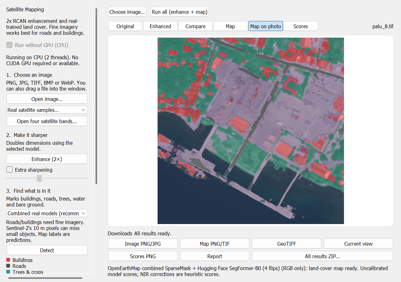
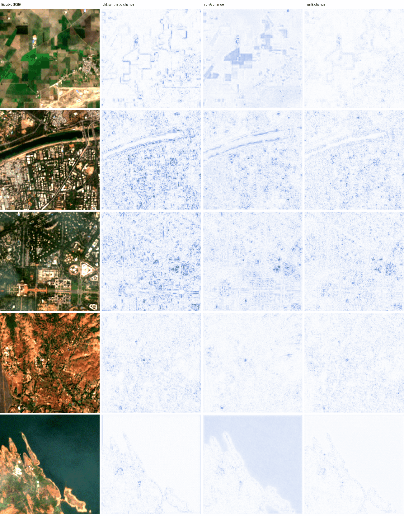
- App changes: a map of where the model changed the image, and exports labelled as model output.
- Repository work: a cleaner package layout, 107 automated tests and a check that runs on every push.
What I built: RCAN trained on real Sentinel-2/VENµS pairs
Oct 2026
The model is a small RCAN: 32 features, 3 groups of 4 blocks, and a shortcut that passes the bicubic image through, so it only learns the correction. It takes 4 colour bands (blue, green, red, near-infrared) and outputs them at twice the size.
For real training pairs I used SEN2VENµS: Sentinel-2 10 m patches matched with same-day 5 m images from the VENµS satellite. I split it by site so no place appears in two splits: 17 sites (41,704 patches) to train on, ALSACE (France) to pick the best version, and BENGA and KUDALIAR (India, 13,039 patches) for the final test.
Two sensor differences had to be handled before training made sense:
- Misregistration. The two satellites’ images are offset by fractions of a 5 m pixel. With a leftover offset, a blurry output scores better than a sharp one, so training rewards blur. I estimate each patch’s shift to 1/8 pixel once, and apply the same shift for every method.
- Contrast. VENµS images have 5–9% less contrast than Sentinel-2 in all four bands. Each reference is rescaled per band to Sentinel-2’s brightness and contrast before training compares against it.
The training loss is the average pixel difference from that aligned, contrast-matched reference, plus a term that keeps the output, shrunk back to 10 m, equal to the input. Training used half-precision numbers to fit an 8 GB laptop GPU, about 3 minutes per pass over the data; the best version came after 5 passes.
The app maps land cover from the original image, not the sharpened one, because the mapping experiment found no benefit from sharpened input. It exports PNG, GeoTIFF, JPEG with location data and a ZIP report. A lighter version runs on ONNX Runtime without PyTorch.
Results: +0.20 dB over bicubic, better on 83% of test patches
Oct 2026
Each method enlarged the 10 m test patches 2x and was scored against the real VENµS 5 m image of the same place and day. A second test shrinks 42 real Indian scenes to 20 m and checks how well each method rebuilds the real 10 m image.
- +0.20 dB PSNR gain over bicubic on 13,039 unseen patches
- 83% of those patches better than bicubic
- 38 / 42 real Indian scenes better than bicubic at reduced scale
| Method | Gain vs bicubic (main score) | Patches better | Reduced-scale test (42 scenes) |
|---|---|---|---|
| Bicubic (40.54 dB) | 0 | n/a | 0 |
| RCAN, artificial training data | −0.26 dB | 2% | −0.63 dB (2 / 42) |
| RCAN, first real run (Run A) | +0.12 dB | 69% | −1.57 dB (0 / 42) |
| ESA SEN2SRLite | −0.04 dB | 31% | −0.12 dB (15 / 42) |
| RCAN, real data (Run B, in the app) | +0.20 dB | 83% | +0.20 dB (38 / 42) |
Three training runs with different random starts agree within ±0.04 dB. The gain is uneven: +0.34 dB at KUDALIAR, +0.03 dB at BENGA, and level with bicubic on ALSACE. With no alignment or contrast corrections at all, the gain is +0.11 dB.
Does it help mapping? I trained the same U-Net mapping model on each kind of input against ESA WorldCover labels at 8 unseen Indian sites, 3 runs each. The original 10 m input scored 47.8% mean IoU; bicubic, RCAN and SEN2SR all scored 48.8–49.3%. Enlarging helps a little, but bicubic already gives that gain, and the differences between methods are smaller than the spread between runs. This ran with the artificially trained RCAN, before retraining.
What broke: the first real-data model flattened every image
- What failed
- Run A, my first model trained on real pairs, scored +0.47 dB over bicubic under my first, more lenient scoring and looked like a success. It was actually copying VENµS’s lower contrast and flattening Sentinel-2 images by 5–25%.
- How I found out
- On the reduced-scale test, which has no VENµS in it, Run A was worse than bicubic on all 42 scenes (−1.57 dB). Its output, shrunk back to 10 m, no longer matched its own input.
- What I changed
- Measured the contrast gap (5–9% in every band), rescaled each reference to Sentinel-2 contrast, estimated each patch’s sub-pixel shift to 1/8 pixel, and retrained on 17 sites (Run B). Withdrew the +0.47 dB figure from the README.
- Still open
- The mapping experiment has not been re-run with Run B. Most of the +0.20 dB comes from one test site, and the main score uses the same contrast correction Run B trained on.
Limits: a small gain, measured honestly
- Small gain. 0.1–0.3 dB is in line with published results for 2x on Sentinel-2. It is not 5 m detail.
- Narrow test. Two test sites, both in India, with very different gains.
- What it measures. VENµS is a different satellite, so the score means “closer to a real 5 m image after correcting known sensor differences”, not recovery of objects smaller than 10 m.
- Mapping labels are 10 m. WorldCover cannot reward detail finer than 10 m, so the mapping test cannot rule out gains that finer labels would show.
- Model output, not measurement. Sharpened images are predictions, and the app’s exports are labelled that way.
References
- Zhang et al., Image super-resolution using very deep residual channel attention networks (RCAN), ECCV 2018
- Michel et al., SEN2VENµS, Data 7(7):96, 2022
- ESA OpenSR: SEN2SR
- ESA WorldCover 2021
- OpenEarthMap
- LoveDA land-cover dataset
Credits. Shantanu Vasagadekar and Shrihari Kshirsagar.
How I used AI tools. Writing boilerplate code and first drafts of the write-ups, to spend more time on the experiments themselves. Every experiment design choice is mine, and every number comes from scripts and raw results in the repository.